OPTPDE - A Collection of Problems in PDE Constrained Optimization

Welcome to the OPTPDE Problem Collection

wavebnd1 details:

Keywords: analytic solution

Global classification: convex

Functional: convex nonlinear

Geometry: easy, fixed

Design: coupled via boundary values 0th order

Differential operator:

Wave:
- linear hyperbolic operator of order 2.
- Defined on a 1-dim domain in 1-dim space
- Time dependent.

Design constraints:

none

State constraints:

box of order 0

Mixed constraints:

none

Description (pdf)
Bibliography (bib)
Problemdata as MATLAB files (tar.gz)

Submitted on 2013-02-07 by Roland Herzog. Published on 2013-02-12

wavebnd1 description:

Introduction

This is an exact controllability problem for the one-dimensional wave equation by Dirichlet boundary actuation. Such problems were thorougly analyzed in Gugat et al. [2005], where the present problem appears as Example 1.

Variables & Notation

Unknowns

\begin{aligned} f_{1}, f_{2} \in L^{\infty} (0, T) & control variables \\ y & state variable \end{aligned}

Given Data

The given data is chosen in a way which admits an analytic solution.

\begin{aligned} y_{0} (x) & = x - 1 ∕ 2 & target displacement \\ y_{1} (x) & = 1 & target velocity \\ T & = 3.25 & ﬁnal time \\ Ω & = (0, 1) & computational domain \\ \hat{r} & = 5 ∕ 28 & auxiliary \\ g_{1} (t) & = - 1 ∕ 4 & auxiliary function \\ g_{2} (t) & = 3 ∕ 4 - t & auxiliary function . \end{aligned}

Problem Description

\begin{aligned} Minimize & \max \{∥ f_{1} ∥_{L^{\infty} (0, T)}, ∥ f_{2} ∥_{L^{\infty} (0, T)} \} \\ s.t. & \{\begin{aligned} y_{t t} & = y_{x x} & in Ω \times (0, T) \\ y (x, 0) & = 0 & in Ω & y_{t} (x, 0) & = 0 & in Ω \\ y (x, T) & = y_{0} (x) & in Ω & y_{t} (x, T) & = y_{1} (x) & in Ω \\ y (0, t) & = f_{1} (t) & in (0, T) & y (1, t) & = f_{2} (t) & in (0, T) . \end{aligned} \end{aligned}

Optimality System

An optimality system is not provided in Gugat et al. [2005] but rather the exact solution is constructed analytically.

Supplementary Material

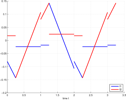
An optimal control can be derived analytically from [Gugat et al., 2005, Theorem 2.2]:

f_{1} (T - t) = \{\begin{matrix} \frac{g_{1} (t) + \hat{r}}{4}, & t \in [0, 0.25] \\ \frac{g_{1} (t) + \hat{r}}{3}, & t \in [0.25, 1] \\ \frac{- g_{2} (t - 1) + \hat{r}}{4}, & t \in [1, 1.25] \\ \frac{- g_{2} (t - 1) + \hat{r}}{3}, & t \in [1.25, 2] \\ \frac{g_{1} (t - 2) + \hat{r}}{4}, & t \in [2, 2.25] \\ \frac{g_{1} (t - 2) + \hat{r}}{3}, & t \in [2.25, 3] \\ \frac{- g_{2} (t - 3) + \hat{r}}{4}, & t \in [3, 3.25] \end{matrix} f_{2} (T - t) = \{\begin{matrix} \frac{g_{2} (t) - \hat{r}}{4}, & t \in [0, 0.25] \\ \frac{g_{2} (t) - \hat{r}}{3}, & t \in [0.25, 1] \\ \frac{- g_{1} (t - 1) - \hat{r}}{4}, & t \in [1, 1.25] \\ \frac{- g_{1} (t - 1) - \hat{r}}{3}, & t \in [1.25, 2] \\ \frac{g_{2} (t - 2) - \hat{r}}{4}, & t \in [2, 2.25] \\ \frac{g_{2} (t - 2) - \hat{r}}{3}, & t \in [2.25, 3] \\ \frac{- g_{1} (t - 3) - \hat{r}}{4}, & t \in [3, 3.25] . \end{matrix}

This pair of optimal controls may not be unique, but it is the unique one with minimal $L^{2} (0, T)$ norm. The corresponding displacement $y$ is piecewise linear, and the optimal velocity $y_{t}$ is piecewise constant on areas bounded by characteristic curves of the equation $y_{t t} = y_{x x}$ . Figure 0.1 displays the optimal controls. A plot of the optimal displacement is provided in [Gugat et al., 2005, Figure 2.1].

Figure 0.1: optimal controls

References

M. Gugat, G. Leugering, and G. Sklyar. $L^{p}$ -optimal boundary control for the wave equation. SIAM Journal on Control and Optimization, 44(1):49–74, 2005. ISSN 0363-0129. doi: 10.1137/S0363012903419212.

Departmentof Mathematics