OPTPDE - A Collection of Problems in PDE Constrained Optimization

Welcome to the OPTPDE Problem Collection

wavebnd2 details:

Keywords: analytic solution

Global classification: linear-quadratic, convex

Functional: convex quadratic

Geometry: easy, fixed

Design: coupled via boundary values 0th order

Differential operator:

Wave:
- linear hyperbolic operator of order 2.
- Defined on a 1-dim domain in 1-dim space
- Time dependent.

Design constraints:

none

State constraints:

linear, local of order 0 at final time
linear, local of order 1 at final time

Mixed constraints:

none

Description (pdf)
Bibliography (bib)
Problemdata as MATLAB files (tar.gz)

Submitted on 2013-03-01 by Martin Gugat. Published on 2013-03-11

wavebnd2 description:

Introduction

Even for smooth data, the optimal state in boundary control problems for the wave equation is in general discontinuous. The continuity of the optimal state can be formulated as an additional requirement. In Gugat [2006], a boundary control problem for the 1D wave equation is considered, with a constraint that the state is at rest at terminal time $T$ . The continuity of the state is achieved by imposing conditions which require the compatibility of the boundary controls with the initial data. Moreover, the objective function (the sum of the $L^{2}$ norms of the time derivatives of the controls) requires the continuity in time of the controls.

This problem and analytical solution appear as [Gugat, 2006, Example 13.2].

Variables & Notation

Unknowns

\begin{aligned} u_{0} \in H^{1} (0, T) & control at the boundary x = 0 \\ u_{L} \in H^{1} (0, T) & control at the boundary x = L \\ y \in H^{1} ((0, L) \times (0, T)) & state variable \end{aligned}

Given Data

The given data is chosen in a way which admits an analytic solution.

\begin{aligned} L & = 1 & length of spatial domain (0, L) \\ T & = 2 & ﬁnal time \\ y_{0} (x) & = - 1 & initial elongation at time zero \\ y_{1} (x) & = 0 & initial velocity at time zero \end{aligned}

Problem Description

\begin{aligned} Minimize & \int_{0}^{T} [u_{0}^{'} {(s)}^{2} + u_{L}^{'} {(s)}^{2}] d s s.t. & \{\begin{aligned} y_{t t} (x, t) & = y_{x x} (x, t) & in (0, L) \times (0, T) \\ y (x, 0) & = y_{0} (x) & in (0, L) \\ y_{t} (x, 0) & = y_{1} (x) & in (0, L) \\ y (0, t) & = u_{0} (t) & in (0, T) \\ y (L, t) & = u_{L} (t) & in (0, T) \\ y (x, T) & = 0 & in (0, L) \\ y_{t} (x, T) & = 0 & in (0, L) \end{aligned} and & \{\begin{aligned} y (0, 0) & = u_{0} (0) \\ y (L, 0) & = u_{L} (0) \\ y (0, T) & = u_{0} (T) \\ y (L, T) & = u_{L} (T) . \end{aligned} \end{aligned}

The state is forced to rest at terminal time $T$ . The ﬁnal block of constraints represents the compatibility conditions which lead to the continuity of the state, together with the continuity of the controls induced by the objective.

Supplementary Material

The optimal controls are given by

u_{0} (t) = u_{L} (t) = - 1 + \frac{t}{2}, t \in [0, T] .

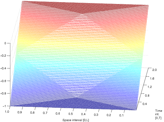
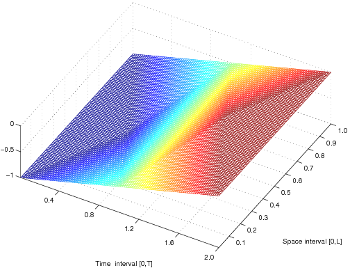
Figure 0.1 shows two views of the optimal state.

Figure 0.1: Optimal state viewed from diﬀerent angles as given in [Gugat, 2006, Figure 1(a) and 1(b)]

The state can be obtained from [Gugat, 2006, Section 11.2.3] as

y (x, t) = \frac{1}{2} [α (x + t) + β (x - t)]

with the functions

\begin{array}{l} α (s) & = \{\begin{matrix} - 1 & s \in [0, 1] \\ s - 2 & s \in [1, 2] \\ 0 & s \in [2, 3] \end{matrix} \\ β (s) & = \{\begin{matrix} 0 & s \in [- 2, - 1] \\ - s - 1 & s \in [- 1, 0] \\ - 1 & s \in [0, 1] . \end{matrix} \end{array}

References

M. Gugat. Optimal boundary control of string to rest in ﬁnite time with continuous state. Zeitschrift für Angewandte Mathematik und Mechanik, 86:134–150, 2006. doi: 10.1002/zamm.200410236.

Departmentof Mathematics