Welcome to the OPTPDE Problem Collection
rddist2 details:
Keywords:
Global classification: nonlinear-quadratic
Functional: convex quadratic
Geometry: easy, fixed
Design: coupled via volume data
Differential operator:
- Schlögel or Nagumo :
- semi-linear parabolic operator of order 2.
- Defined on a 1-dim domain in 1-dim space
- Time dependent.
Design constraints:
- none
State constraints:
- none
Mixed constraints:
- none
Submitted on 2013-05-24 by Fredi Tröltzsch. Published on 2013-05-21
rddist2 description:
Introduction
This is a distributed optimal control problem for a semilinear 1D parabolic reaction-diffusion equation, where traveling wave fronts occur. The state equation is known as Schlögl model in physics and as Nagumo equation in neurobiology. In this context, various goals of optimization are of interest, for instance the stopping, acceleration, or extinction of a traveling wave. Here, we discuss the problem of re-directing a wave front after a certain time. The control is acting only on two subdomains near the boundary, which occupy the portion of the entire spatial domain. This problem appears in [Buchholz et al., 2013, Section 5.2]. In the same paper, additional examples can be found which cover the other optimization goals mentioned above.
Variables & Notation
Unknowns
Given Data
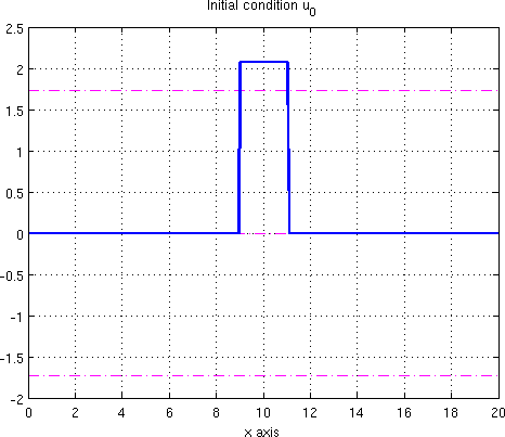
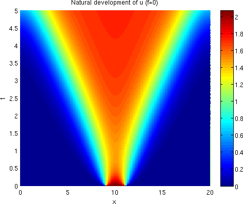
The natural uncontrolled state is shown in Figure 0.1. In the figure, the horizontal axis shows the spatial variable while the vertical one displays the time . The speed of the uncontrolled wave front was determined numerically.
Problem Description
Notice that the PDE has a non-monotone nonlinearity. The associated homogeneous elliptic (stationary) equation admits three different solutions; namely, the functions , , and .
Optimality System
The following optimality system for the state , the control , and the adjoint state , given in the strong form, represents first-order necessary optimality conditions.
Supplementary Material
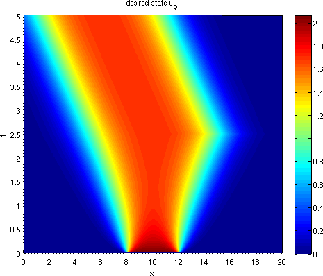
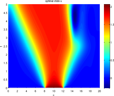
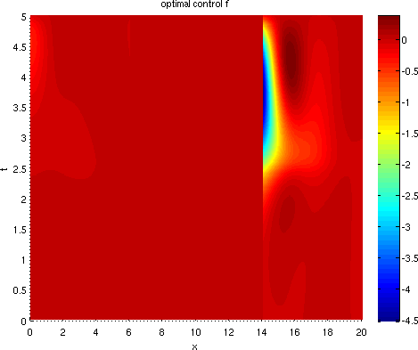
Figure 0.2 displays the desired state, as well as the optimal state and optimal control.
References
R. Buchholz, H. Engel, E. Kammann, and F. Tröltzsch. On the optimal control of the Schlögl model. Computational Optimization and Applications, 56(1):153–185, 2013. doi: 10.1007/s10589-013-9550-y.