Welcome to the OPTPDE Problem Collection
ccparfin1 details:
Keywords: analytic solution
Global classification: nonlinear-quadratic
Functional: convex quadratic
Geometry: easy, fixed
Design: coupled via volume data
Differential operator:
- Heat:
- semi-linear parabolic operator of order 2.
- Defined on a 2-dim domain in 2-dim space
- Time dependent.
Design constraints:
- box of order 0
State constraints:
- none
Mixed constraints:
- none
Submitted on 2013-05-27 by Fredi Tröltzsch. Published on 2013-06-21
ccparfin1 description:
Introduction
This example is an optimal control problem for a semilinear heat equation with cubic nonlinearity in a two dimensional domain. There are four time-dependent control functions restricted by box constraints. The example is constructed such that a locally optimal solution is explicitly known. It was used in the context of model reduction by POD to test an a posteriori error estimator for optimality, and appears in [Kammann et al., 2013, Section 4.2].
Variables & Notation
Unknowns
Given Data
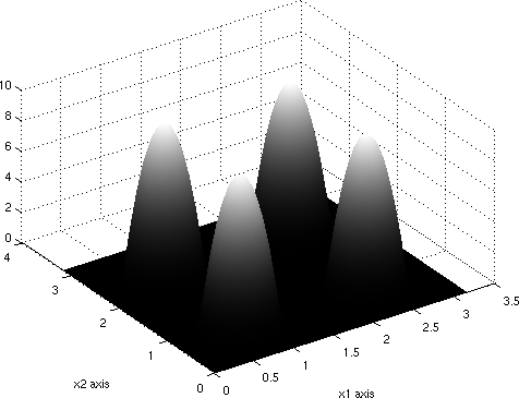
The graphs of the functions are shown in Figure 0.1.
Problem Description
Optimality System
The following optimality system for the state , the control , and the adjoint state , given in the strong form, represents first-order necessary optimality conditions.
Supplementary Material
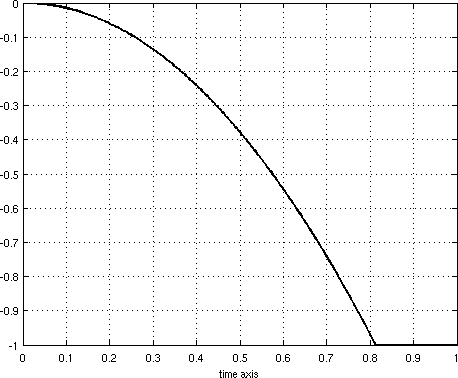
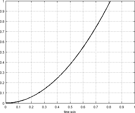
A set of locally optimal controls with associated state and adjoint state are known analytically.
The controls are shown in Figure 0.2.
To show the local optimality of this solution, we verify that obeys the standard second-order sufficient optimality conditions.1 1 This analysis is not presented in Kammann et al. [2013] but it was carried out by the authors in 2014 (unpublished). To this end, we introduce the Lagrangian; writing , we define
Notice that and is satisfied. Invoking [Tröltzsch, 2010, Theorem 5.17], we obtain that is locally optimal with respect to the topology of . (The quoted theorem is formulated for a control function , but it obviously extends to the case .)
Revision History
- 2016–06–10: added comment on second-order sufficient conditions
- 2014–10–30: formulas for the control weights corrected to match the calculations and figures in [Kammann et al., 2013, Section 4.2]
- 2013–05–27: problem added to the collection
References
E. Kammann, F. Tröltzsch, and S. Volkwein. A posteriori error estimation for semilinear parabolic optimal control problems with application to model reduction by POD. ESAIM. Mathematical Modelling and Numerical Analysis, 47(2):555–581, 2013. ISSN 0764-583X. doi: 10.1051/m2an/2012037.
F. Tröltzsch. Optimal Control of Partial Differential Equations, volume 112 of Graduate Studies in Mathematics. American Mathematical Society, Providence, 2010.