Departmentof Mathematics

Introduction

This is a semilinear elliptic optimal control problem with a nonsmooth PDE constraint. The problem presented here is case 2 in Weiß et al. [2019], where an efficient numerical solution method, named SCALi, is presented as well. The problem class considered in Weiß et al. [2019] contains elliptic PDE constraints with a nonsmooth semilinear part consisting of a combination of differentiable superposition operators and the absolute value function. The present problem is special in the sense that the desired state is not a feasible solution. Moreover, the control to state operator is nonsmooth due to the nonsmoothness in the state equation. Hence, standard techniques for obtaining first order minima can not be applied.

Variables & Notation

Unknowns

$$\begin{array}{ccc}\hfill u\in L^2\left(\Omega \right)& \text{control variable}\hfill & \hfill \\ \hfill y\in H_0^1\left(\Omega \right)& \text{state variable}\hfill \end{array}$$

Given Data

The given data is chosen in a way which allows for comparatively easy implementation but the desired state should not be achievable.

$$\begin{array}{llllllll}\hfill \Omega & ={\left(0,1\right)}^2& \hfill & \text{computational domain}& \hfill & & \hfill & \\ \hfill \Gamma & & \hfill & \text{its boundary}& \hfill & & \hfill & \\ \hfill y_d\left(x_1,x_2\right)& =\frac{\sin <!--FUNCTION\; APPLICATION-->\left(\right.10\pi \left({\left(x_1-\frac{1}{2}\right)}^2+{\left(x_2-\frac{1}{2}\right)}^2\right)\left)\right.}{\sqrt{\frac{1}{100}+{\left(x_1-\frac{1}{2}\right)}^2+{\left(x_2-\frac{1}{2}\right)}^2}}-1& \hfill & \text{desired state}& \hfill & & \hfill & \\ \hfill \ell \left(y\right)& =\max <!--FUNCTION\; APPLICATION-->\left(5y,y\left|y\right|\right)& \hfill & \text{nonlinear nonsmooth operator}& \hfill & & \hfill & \end{array}$$

---

---

Note that the nonlinearity $\ell$ can be rewritten as follows

$$\ell \left(y\right)=\max <!--FUNCTION\; APPLICATION-->\left(5y,y\left|y\right|\right)=\frac{1}{2}\left(5y+y\left|y\right|+\left|5y-y\left|y\right|\right|\right).$$

Problem Description

$$\begin{array}{llll}\hfill \text{Minimize}& \frac{1}{2}\parallel y-y_d{\parallel }_{L^2}^2+\frac{\alpha }{2}\parallel u{\parallel }_{L^2}^2& \hfill & \\ \hfill \text{s.t.}& \left\{\begin{array}{ccccc}\hfill -△y+\ell \left(y\right)& =u\hfill & \hfill & \text{in }\Omega ,\hfill & \hfill \\ \hfill y& =0\hfill & \hfill & \text{on }\partial \Omega .\hfill \end{array}\right.& \hfill & \end{array}$$

Supplementary Material

In Weiß et al. [2019] this problem was treated with a special handling of the absolute value operator based on the abs-linearization. Using the resulting algorithm SCALi the numerical results presented in Table 0.1 were obtained, considering different values of the mesh size denoted by $h$ and the penalty parameter $\alpha$ for the control in the objective functional. For the computations the starting values $y\equiv 0$ and $u\equiv 0$ where taken.

Note that in this demanding case, where a genuine non-linear and non-smooth operator in the PDE and an unreachable target function $y_d$ occur, comparatively more Newton iterations are needed to compute the minimal solution, see Weiß et al. [2019].

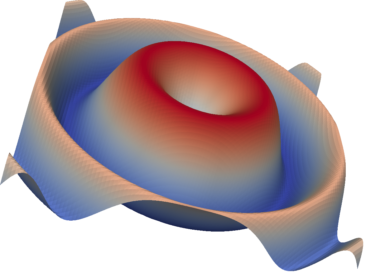
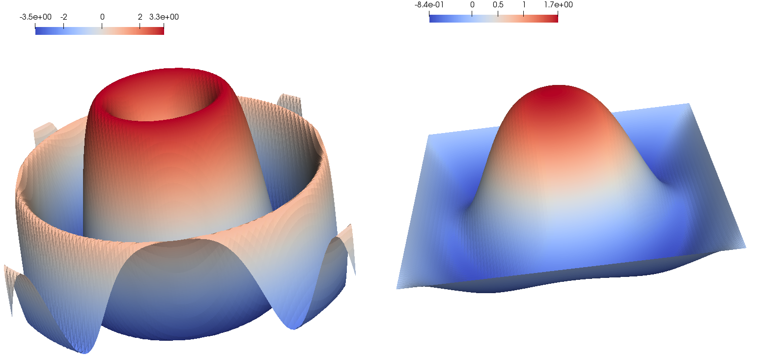
Figure 0.2 shows the desired state $y_d$ and the solution state corresponding to the parameters given in the first row in Tab. 0.1.

---

---

For the numerical results, a Finite-Element-Approach within the open source finite element environment FEniCS (c.f. Logg et al. [2012]) to discretize the PDE in combination with a Newton method for the solution of smooth modified branch problems according to the algorithm SCALi (c.f. Weiß et al. [2019]) was used.

All calculations were performed with FEniCS, version 2019.1.0, using the Python interface.

References

A. Logg, G. Wells, and K Mardel. Automated Solution of Differential Equations by the Finite Element Method, volume 84 of Lecture Notes in Computational Science and Engineering. Springer Berlin Heidelberg, Berlin, Heidelberg, 2012.
O. Weiß, S. Schmidt, and A. Walther. Solving non-smooth semi-linear elliptic optimal control problems with abs-linearization. Technical report, Optimization Online, 2019. URL http://www.optimization-online.org/DB_HTML/2018/10/6890.html.