Departmentof Mathematics

Introduction

We consider the optimal control of static elastoplasticity with linear kinematic hardening. This leads to an optimal control problem governed by an elliptic variational inequality of first kind in mixed form or, equivalently, an MPCC in function space.
The objective functional tracks the state both on the entire domain and additionally on a submanifold of the domain. The control cost is taken into account by a tracking type term as well. There are no constraints on the control, which acts in a distributed way on the domain. The Dirichlet boundary is the entire boundary of the domain.
A locally optimal control is known, whose corresponding state has a bi-active set with a positive measure.

The problem and its solution are taken from [Betz et al., 2014, Section 6.1].

Variables & Notation

Unknowns

The state is composed of the stress $\sigma$, back stress $\chi$, displacement $u$ and plastic multiplier $\lambda$.

Given Data

desired displacement in the domain:

with

desired displacement on the submanifold $\partial B$:

desired control:

Problem Description

With the given Lamé coefficients, the inverse elasticity and hardening tensors read

where $I:{ℝ}_{\text{sym}}^{2\times 2}\to {ℝ}_{\text{sym}}^{2\times 2}$ is the identity mapping and

The yield function is given by

where $\parallel \cdot {\parallel }_F$ denotes the Frobenius norm of a matrix. The corresponding inner product $\mathrm{trace}<!--FUNCTION\; APPLICATION-->\left(A^{\top <!--FUNCTION\; APPLICATION-->}B\right)$ is used in the calculation of ${\left(\cdot ,\cdot \right)}_{L^2\left(\Omega ;{ℝ}_{\text{sym}}^{2\times 2}\right)}$.

Optimality System

According to [Betz and Meyer, 2015, Theorem 4.6] (Theorem 4.4 in the Preprint) the following conditions are sufficient for local optimality of the control $f$ with associated state $\left(\right.\sigma ,\chi ,u,\lambda \left)\right.$.
There exist adjoint variables $\left(\right.\zeta ,\psi ,w\left)\right.\in L^{\infty }\left(\right.\Omega ;{ℝ}_{\text{sym}}^{2\times 2}{\left)\right.}^2\times H_0^1\left(\right.\Omega ;{ℝ}^2\left)\right.$ and multipliers $\left(\mu ,𝜃\right)\in L^{\infty }\left(\Omega \right)\times L^{\infty }\left(\Omega \right)$ satisfying

1. the optimality system $$\begin{array}{llll}\hfill {ℂ}^{-1}\zeta -𝜀\left(w\right)+\lambda \left(\right.{\zeta }^D+{\psi }^D\left)\right.+𝜃\left(\right.{\sigma }^D+{\chi }^D\left)\right.& =0\text{in }{L}^2\left(\right.\Omega ;{ℝ}_{\text{sym}}^{2\times 2}\left)\right.& \hfill & \\ \hfill {ℍ}^{-1}\psi +\lambda \left(\right.{\zeta }^D+{\psi }^D\left)\right.+𝜃\left(\right.{\sigma }^D+{\chi }^D\left)\right.& =0\text{in }{L}^2\left(\right.\Omega ;{ℝ}_{\text{sym}}^{2\times 2}\left)\right.& \hfill & \\ \hfill -\left(\right.\zeta ,𝜀\left(v\right){\left)\right.}_{L^2\left(\Omega ;{ℝ}_{\text{sym}}^{2\times 2}\right)}+{\left(u-u_{\Omega },v\right)}_{L^2\left(\Omega ;{ℝ}^2\right)}& & \hfill & \\ \hfill +{\left(u-u_{\partial B},v\right)}_{L^2\left(\partial B;{ℝ}^2\right)}& =0\forall <!--FUNCTION\; APPLICATION-->v\in H_0^1\left(\right.\Omega ;{ℝ}^2\left)\right.& \hfill & \\ \hfill w+\alpha \left(f-f_{\Omega }\right)& =0\text{in }{L}^2\left(\right.\Omega ;{ℝ}^2\left)\right.& \hfill & \\ \hfill \left(\right.{\sigma }^D+{\chi }^D\left)\right.:\left(\right.{\zeta }^D+{\psi }^D\left)\right.-\mu & =0\text{a.e. in }\Omega & \hfill & \\ \hfill \mu \lambda & =0\text{a.e. in }\Omega & \hfill & \\ \hfill 𝜃\varphi \left(\sigma ,\chi \right)& =0\text{a.e. in }\Omega & \hfill & \\ \hfill \mu & \ge 0\text{a.e. in }\Omega & \hfill & \\ \hfill 𝜃& \ge 0\text{a.e. in }\Omega & \hfill & \end{array}$$
2. the second-order condition
   There exists $\kappa >0$ such that

   $${\partial }_{\left(\sigma ,\chi ,u,\lambda ,f\right)}^2\mathcal{ℒ}\left(\right.\sigma ,\chi ,u,\lambda ,f,\zeta ,\psi ,w,\mu ,𝜃\left)\right.\left(\right.{\sigma }^{\prime },{\chi }^{\prime },u^{\prime },{\lambda }^{\prime },h{\left)\right.}^2\ge \kappa \parallel h{\parallel }_U^2$$

   holds for all $h\in L^2\left(\right.\Omega ;{ℝ}^2\left)\right.$ and $\left(\right.{\sigma }^{\prime },{\chi }^{\prime },u^{\prime },{\lambda }^{\prime }\left)\right.$ solving

   $$\begin{array}{llll}\hfill {ℂ}^{-1}{\sigma }^{\prime }-𝜀\left(u^{\prime }\right)+\lambda \left(\right.{\left({\sigma }^{\prime }\right)}^D+{\left({\chi }^{\prime }\right)}^D\left)\right.+{\lambda }^{\prime }\left(\right.{\sigma }^D+{\chi }^D\left)\right.& =0\text{in }{L}^2\left(\right.\Omega ;{ℝ}_{\text{sym}}^{2\times 2}\left)\right.& \hfill & \\ \hfill {ℍ}^{-1}{\chi }^{\prime }+\lambda \left(\right.{\left({\sigma }^{\prime }\right)}^D+{\left({\chi }^{\prime }\right)}^D\left)\right.+{\lambda }^{\prime }\left(\right.{\sigma }^D+{\chi }^D\left)\right.& =0\text{in }{L}^2\left(\right.\Omega ;{ℝ}_{\text{sym}}^{2\times 2}\left)\right.& \hfill & \\ \hfill -\left(\right.{\sigma }^{\prime },𝜀\left(v\right){\left)\right.}_{L^2\left(\Omega ;{ℝ}_{\text{sym}}^{2\times 2}\right)}+{\left(h,v\right)}_{L^2\left(\Omega ;{ℝ}^2\right)}& =0\forall <!--FUNCTION\; APPLICATION-->v\in H_0^1\left(\right.\Omega ;{ℝ}^2\left)\right.& \hfill & \\ \hfill ℝ\ni {\lambda }^{\prime }\perp \left(\right.{\sigma }^D+{\chi }^D\left)\right.:\left(\right.{\left({\sigma }^{\prime }\right)}^D+{\left({\chi }^{\prime }\right)}^D\left)\right.& =0\text{a.e. in }{\mathcal{𝒜}}_s& \hfill & \\ \hfill 0\le {\lambda }^{\prime }\perp \left(\right.{\sigma }^D+{\chi }^D\left)\right.:\left(\right.{\left({\sigma }^{\prime }\right)}^D+{\left({\chi }^{\prime }\right)}^D\left)\right.& \le 0\text{a.e. in }\mathcal{ℬ}& \hfill & \\ \hfill 0={\lambda }^{\prime }\perp \left(\right.{\sigma }^D+{\chi }^D\left)\right.:\left(\right.{\left({\sigma }^{\prime }\right)}^D+{\left({\chi }^{\prime }\right)}^D\left)\right.& \in ℝ\text{a.e. in }\mathcal{ℐ}.& \hfill & \end{array}$$

   The sets are defined as follows,

   $$\begin{array}{ccccc}\hfill {\mathcal{𝒜}}_s& :=\left\{x\in \Omega :\lambda >0\right\}\hfill & \hfill & \text{strongly active set},\hfill & \hfill \\ \hfill \mathcal{ℬ}& :=\left\{x\in \Omega :\varphi \left(\sigma ,\chi \right)=\lambda =0\right\}\hfill & \hfill & \text{bi-active set},\hfill \\ \hfill \mathcal{ℐ}& :=\left\{x\in \Omega :\varphi \left(\sigma ,\chi \right)<0\right\}\hfill & \hfill & \text{inactive (elastic) set},\hfill \end{array}$$

   and the Lagrangian $\mathcal{ℒ}$ is defined by

   $$\begin{array}{ccc}\hfill & \mathcal{ℒ}\left(\sigma ,\chi ,u,\lambda ,f,\zeta ,\psi ,w,\mu ,𝜃\right)\hfill & \hfill \\ \hfill & =J\left(u,f\right)+\left(\right.\sigma -𝜀\left(u\right)+\lambda \left(\right.{\sigma }^D+{\chi }^D\left)\right.,\zeta {\left)\right.}_{L^2\left(\Omega ;{ℝ}_{\text{sym}}^{2\times 2}\right)}\hfill \\ \hfill & +\left(\right.\chi +\lambda \left(\right.{\sigma }^D+{\chi }^D\left)\right.,\psi {\left)\right.}_{L^2\left(\Omega ;{ℝ}_{\text{sym}}^{2\times 2}\right)}-\left(\right.\sigma ,𝜀\left(w\right){\left)\right.}_{L^2\left(\Omega ;{ℝ}_{\text{sym}}^{2\times 2}\right)}\hfill \\ \hfill & +{\left(f,w\right)}_{L^2\left(\Omega ;{ℝ}^2\right)}-{\left(\lambda ,\mu \right)}_{L^2\left(\Omega \right)}+{\left(\varphi \left(\sigma ,\chi \right),𝜃\right)}_{L^2\left(\Omega \right)}.\hfill \end{array}$$

   Consequently ${\partial }_{\left(\sigma ,\chi ,u,\lambda ,f\right)}^2\mathcal{ℒ}\left(\right.\sigma ,\chi ,u,\lambda ,f,\zeta ,\psi ,w,\mu ,𝜃\left)\right.\left(\right.{\sigma }^{\prime },{\chi }^{\prime },u^{\prime },{\lambda }^{\prime },h{\left)\right.}^2$ is given as follows:

   $$\begin{array}{ccc}\hfill {\partial }_{\left(\sigma ,\chi ,u,\lambda ,f\right)}^2& \mathcal{ℒ}\left(\right.\sigma ,\chi ,u,\lambda ,f,\zeta ,\psi ,w,\mu ,𝜃\left)\right.\left(\right.{\sigma }^{\prime },{\chi }^{\prime },u^{\prime },{\lambda }^{\prime },h{\left)\right.}^2\hfill & \hfill \\ \hfill & ={\left(u^{\prime },u^{\prime }\right)}_{L^2\left(\Omega ;{ℝ}^2\right)}+{\left(u^{\prime },u^{\prime }\right)}_{L^2\left(\partial B;{ℝ}^2\right)}+\alpha {\left(h,h\right)}_{L^2\left(\Omega ;{ℝ}^2\right)}\hfill \\ \hfill & +2\left(\right.{\lambda }^{\prime }\left(\right.{\left({\sigma }^{\prime }\right)}^D+{\left({\chi }^{\prime }\right)}^D\left)\right.,{\zeta }^D+{\psi }^D{\left)\right.}_{L^2\left(\Omega ;{ℝ}_{\text{sym}}^{2\times 2}\right)}\hfill \\ \hfill & +\left(\right.∥{\left({\sigma }^{\prime }\right)}^D+{\left({\chi }^{\prime }\right)}^D{∥}_F^2,𝜃{\left)\right.}_{L^2\left(\Omega \right)}.\hfill \end{array}$$

Supplementary Material

Locally optimal control, state, adjoint state and multipliers are known analytically:

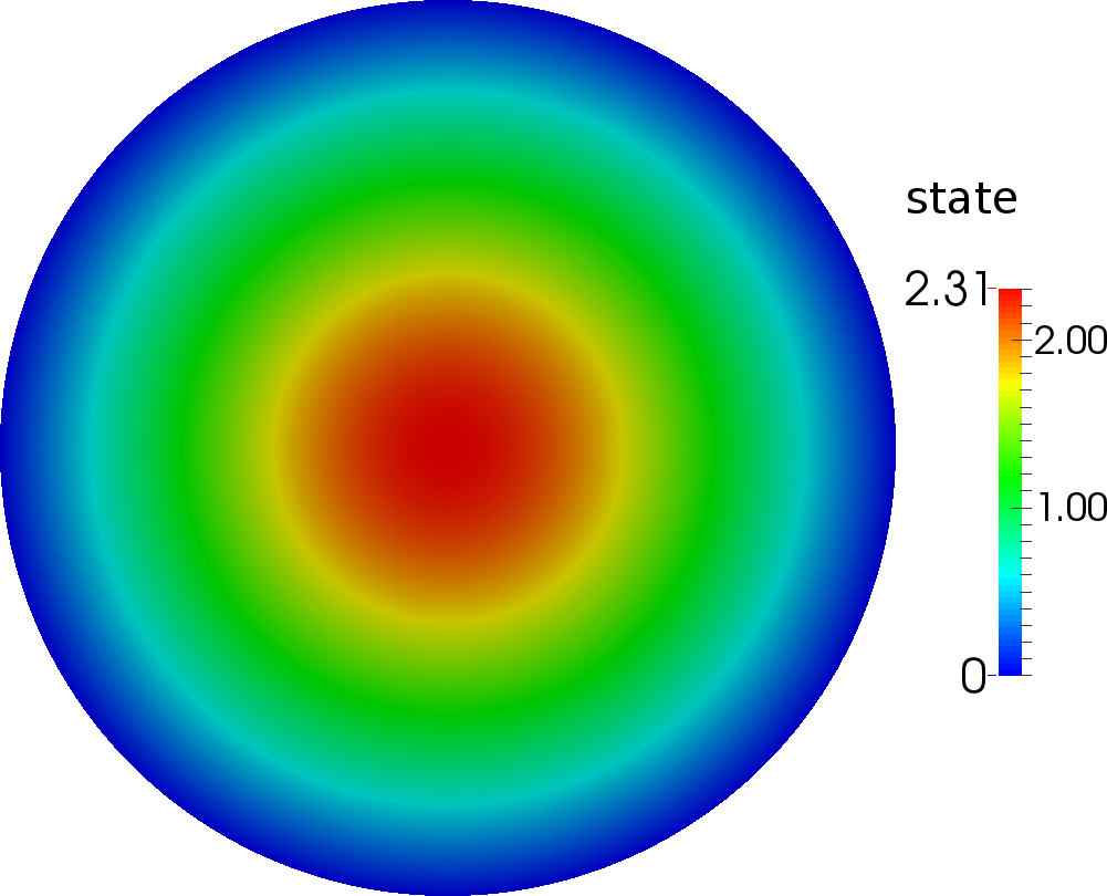
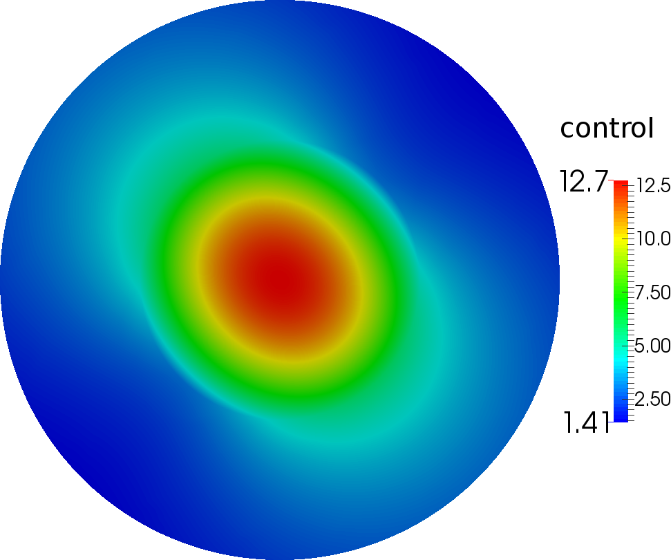
The magnitude of the optimal state and control for the values $\alpha =1$ and ${\sigma }_0=2$ as given in Betz et al. [2014] are depicted in Figure 0.1. The reference value for the objective,

corresponding to these values of $\alpha$ and ${\sigma }_0$ is given in Betz et al. [2014].

Revision History

• 2015–04–22: Updated reference to the published version.
• 2014–11–29: Explicit formulas for the second-order derivative of the Lagrangian added. Formulas for optimal $\sigma$ and $f$ added. Pictures of the optimal solution added. Reference for objective value added. Matlab code added.
• 2014–04–23: problem added to the collection

References

T. Betz and C. Meyer. Second-order sufficient optimality conditions for optimal control of static elastoplasticity with hardening. ESAIM: Control, Optimisation and Calculus of Variations, 21(1):271–300, 2015. doi: 10.1051/cocv/2014024.
T. Betz, C. Meyer, A. Rademacher, and K. Rosin. Adaptive optimal control of elastoplastic contact problems. Technical report, Fakultät für Mathematik, TU Dortmund, May 2014. URL http://www.mathematik.tu-dortmund.de/papers/BetzMeyerRademacherRosin2014.pdf. Ergebnisberichte des Instituts für Angewandte Mathematik, Nummer 496.